
Linking obligor-specific data to individual municipal bond securities
ICE Climate links hundreds of thousands of individual securities to the geospatial footprints of their obligors. Our geospatial downscaling and re-aggregation approach takes us one step further. It allows us to infer obligor-specific information about socioeconomic, education, employment, and health characteristics, as well as hazard and extreme weather risk.
Published
September 2024
Every week, towns, cities, counties, special districts, utility companies, and states issue municipal bonds to raise funds for infrastructure projects. Many of these bonds are secured by taxes or other revenue generated from the residents and customers within the geographic boundary of the obligated municipality, district, or utility. In a previous article, ICE Climate introduced our geospatial library of municipal bond obligor-issuer pairs — a library that allows us link more than 90% of outstanding municipal debt to specific geospatial boundaries.
However, making the link between geospatial boundaries and securities represents only a piece of the puzzle, because ICE Climate also aims to provide information on socioeconomic, education, employment, health, and hazard and extreme weather risk for obligated communities across the county. Our main data sources include the U.S. Census, the Centers for Disease Control, the U.S. Environment Protection Agency (EPA), the Bureau of Labor Statistics, and the Federal Emergency Management Agency (FEMA) — agencies that generally provide data at the level of census tracts and counties.
Figure 1. (left) The boundary of Sacramento County, California. (center) The boundary of Sacramento County, California, with 2020 census tract boundaries shown in black. (right) Same map as the center, but census tracts shaded by U.S. Census data on the populations within each tract in 2020.
The challenge is this: The boundaries of municipalities and other municipal bond obligors do not necessarily align with census tracts and counties. For example, a utility district like the Sacramento County Water Agency (Lagune-Vineyard) spans and cuts across many census tracts (Figure 2). Larger utility service areas (Pacific Gas and Electric, for example) can span many counties, and some utilities can even straddle state boundaries. In many cases, school districts, towns, villages, and fire district boundaries also cross-cut census tracts (Figure 2).
Figure 2. Obligor boundaries (as well as other areas that may be of interest) often do not align perfectly with census tracts or countries. Within Sacramento County (black outline), school districts and utilities often cut across multiple tracts.
In other cases, a municipal bond obligor may be a community facilities district or special development district that is only a few hundred yards across, wholly contained within a single tract (Figure 3).
Figure 3. Obligor boundaries can also be smaller than tracts, like the two small community facilities districts highlighted in yellow on the left.
To provide accurate information about the communities living within obligor boundaries across the country, ICE Climate uses a rigorous downscaling and re-aggregation methodology to make inferences based on tract- and county-level data. This approach takes advantage of sophisticated geospatial weighting schemes that incorporate higher resolution data.
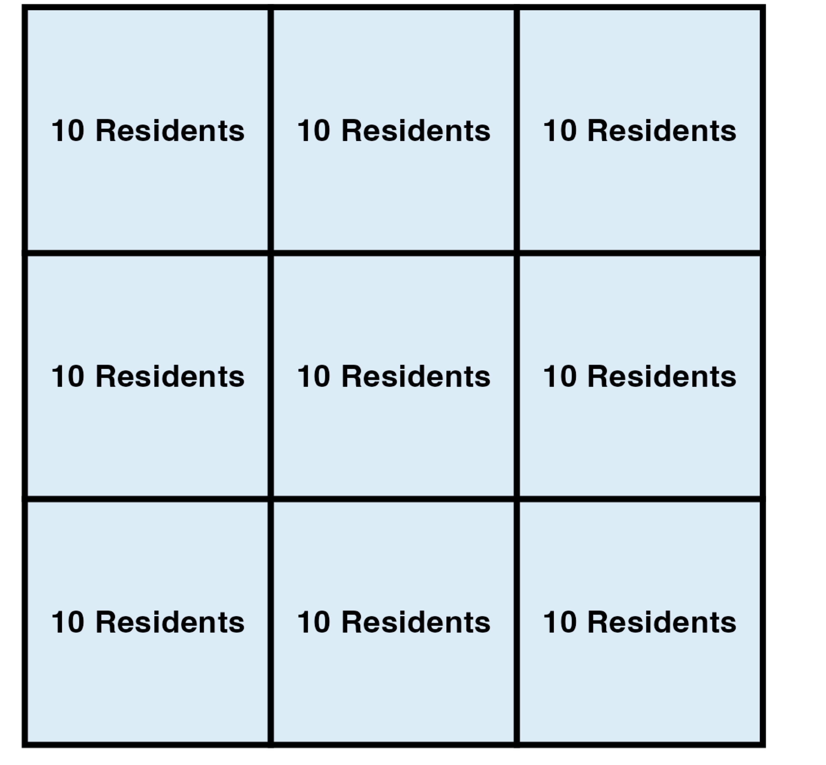
What does this mean? Let’s take a simple example. Imagine a hypothetical square land area with a total population of 90 people.
In the absence of other information, we could assume that the population is evenly distributed across the area.
This is a reasonable first assumption—but if we had additional information at a higher resolution (9 smaller areas within the single larger area), like the distribution of residential properties, we could refine our inference even further.
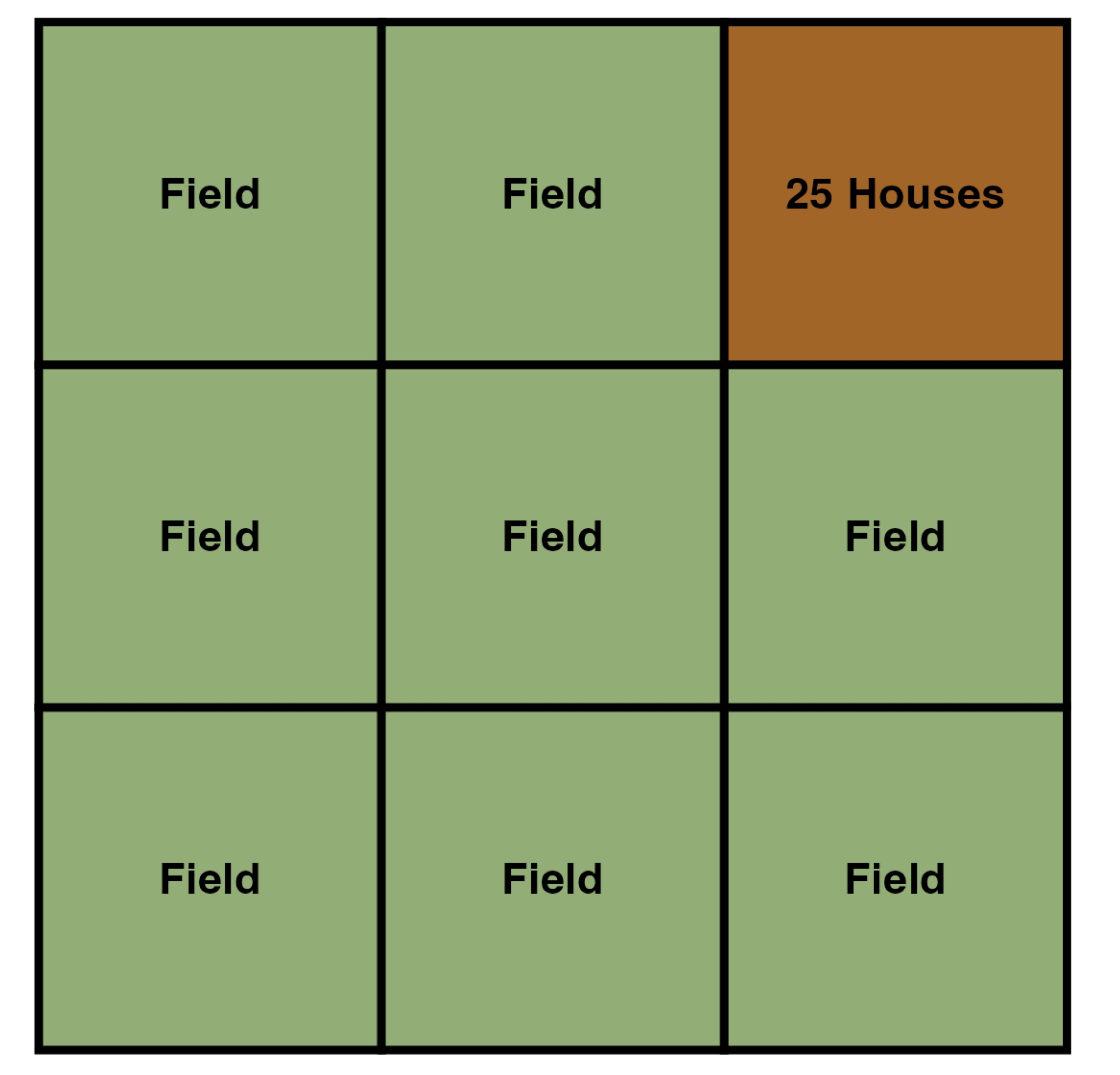
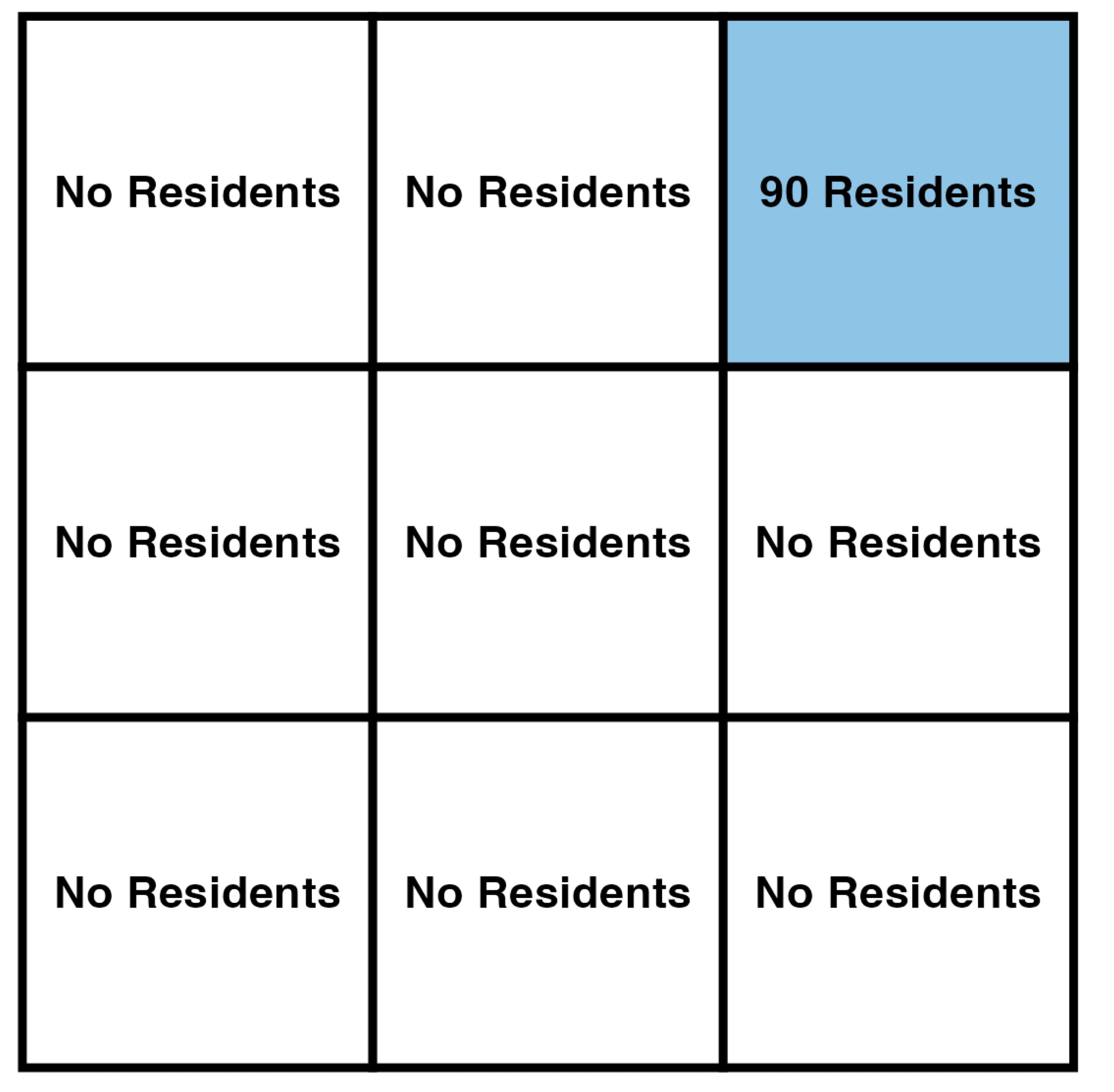
For example, if we knew that all the houses in the area were in one corner, and the rest of the area was a grassy field, we could reasonably infer that the entire population resides within a much smaller area.
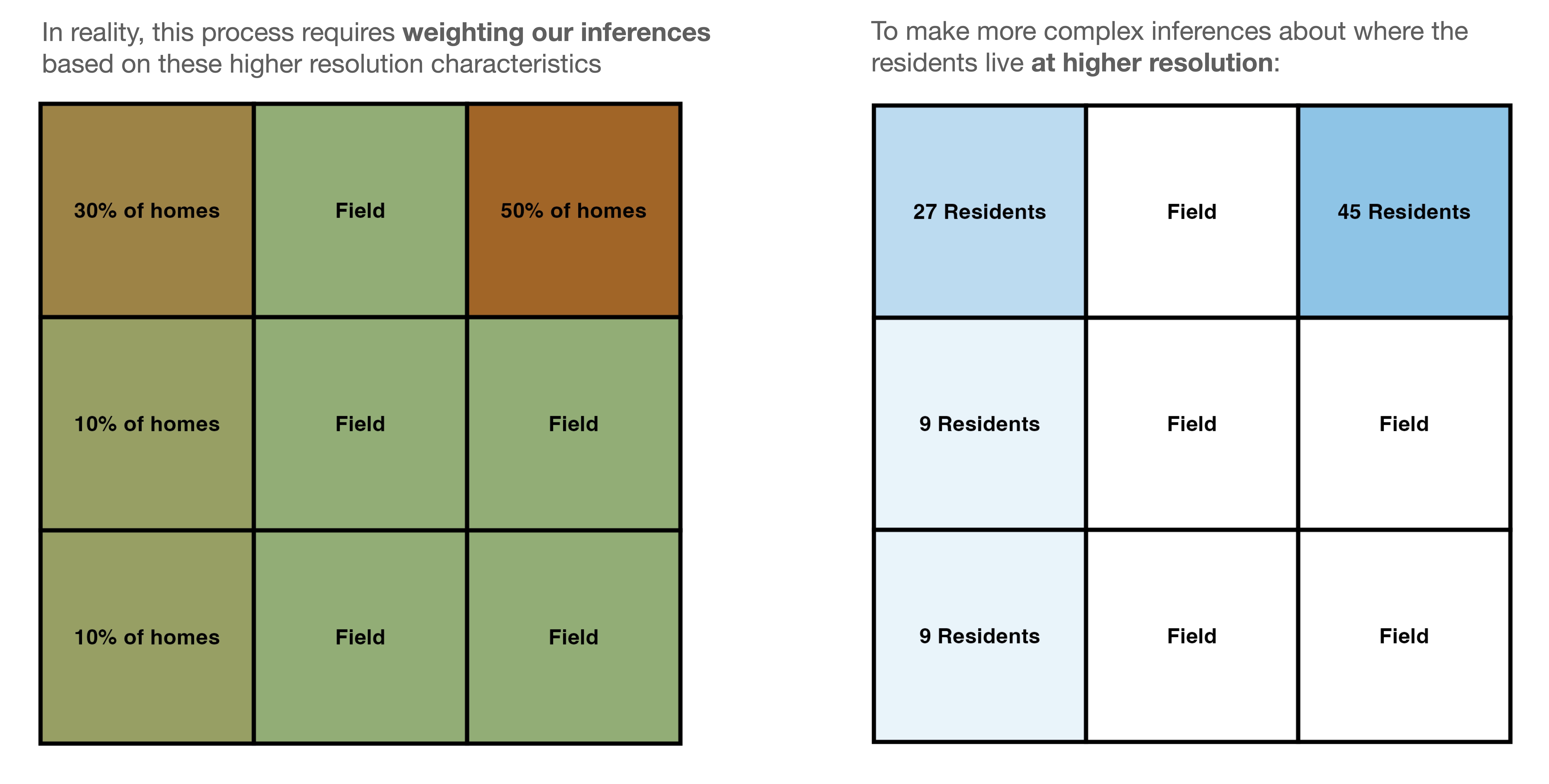
In reality, this process is much more complex. For one thing, it is rare that all residents of an area live in one specific sub-region. Therefore, in practice, we use high resolution data to create weights (geographers and demographers call these ‘dasymetic weights’) with which we can intelligently downscale information that comes at a course scale (i.e., a total of 90 residents live in a large land area) onto a finer grid (the residents actually live in a small subset of that area).
To take our same example, if we knew that 50% of residential properties within the land area were in the upper-right corner, while the remaining 10%, 10% and 30% of residential properties were located along the lefthand side of the area, we would infer that the population is distributed accordingly.
This approach can be extended beyond population, to other types of information. For example, imagine we had two adjoining census tracts, each with 90 residents. In one tract, the U.S. Census reports that 30% of the population has access to regular preventative medical care; in the other, the U.S. Census reports that 70% has access to regular preventative medical care. Imagine a medical group with a coverage region that spans two-thirds of the area of each tract (the obligor boundary in blue, below).
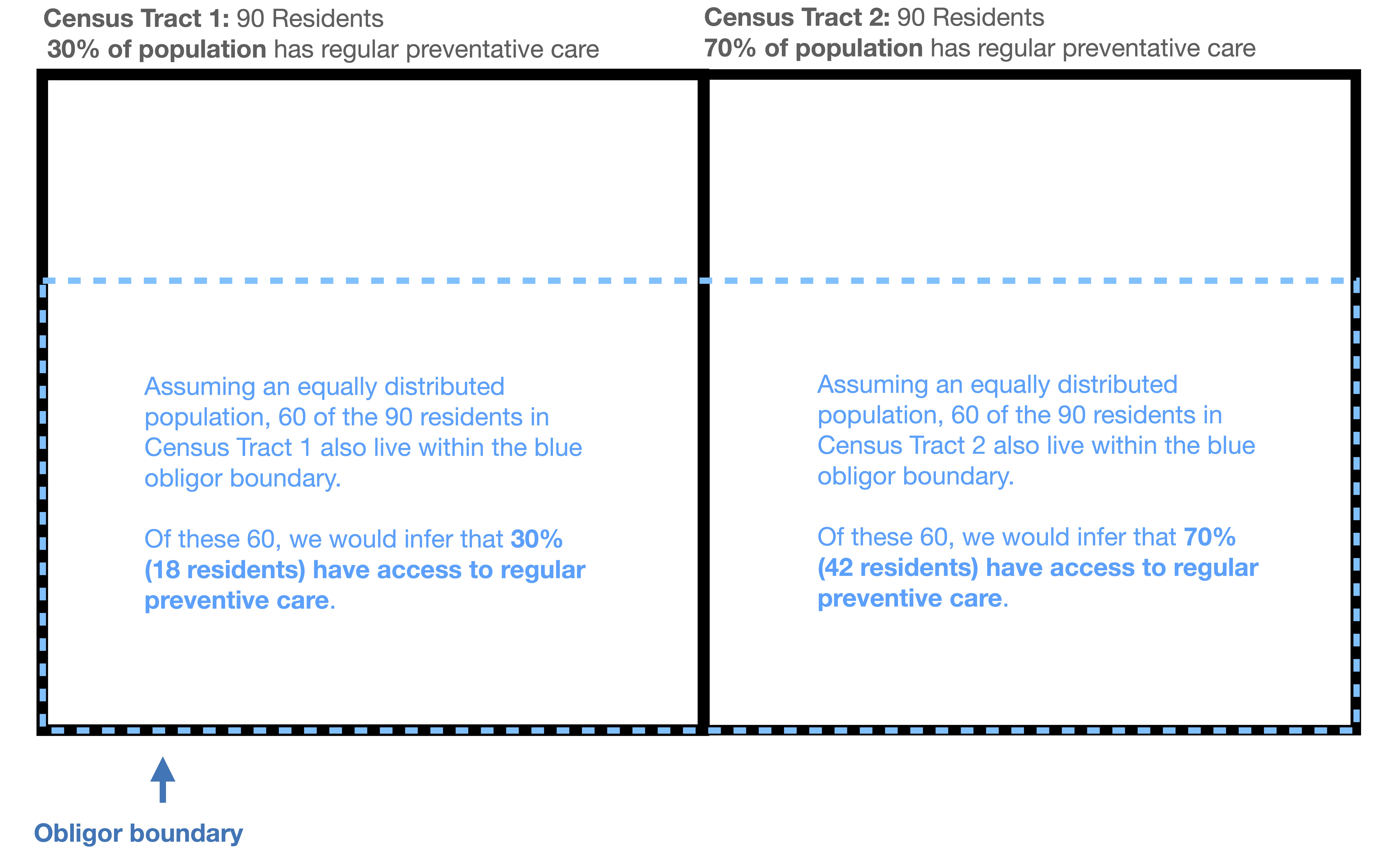
To infer the percentage of the population that has regular preventative care within the medical group’s coverage area (blue boundary), we could make the naïve assumption that the population in each tract is evenly distributed. Under this assumption, we would infer that 60 of the 90 residents of Census Tract 1 live within the blue obligor boundary, and 30% of these 60 people (18 residents) have access to regular medical care. In Census Tract 2, we would again infer that 60 of 90 tract residents live within the blue boundary—but in this tract’s case, 70% of the 60 (42 residents) have access to regular preventative care. This approach would lead us to conclude that of the 120 total residents living within the blue boundary across both tracts, 60 residents, or 50% of them (18 people in tract 1 and 42 people in tract 2) likely have access to regular preventative care.
However, additional information can help us to refine this inference even further. The diagram below suggests that only 20% of residential properties within the blue obligor boundary are in Census Tract 1, and the remaining 80% are in Census Tract 2.
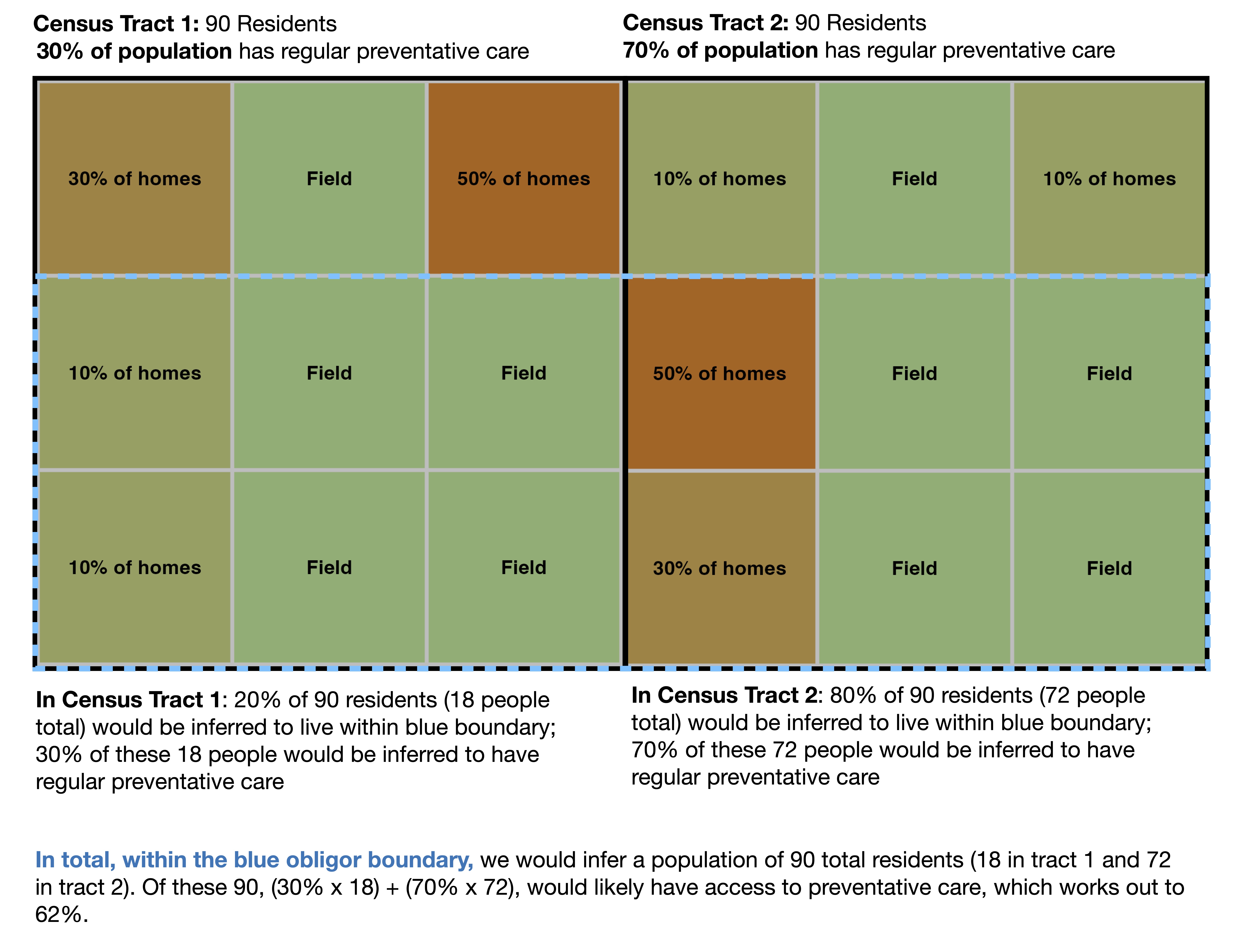
We can weight our inference of the percentage of the population with regular preventative care accordingly. Within the blue boundary, we would infer a total population of 90 residents (18 in tract 1 and 72 in tract 2). Of these 90 residents, the number inferred to have access to regular preventative care would be: (30% access x 18 residents of tract 1) + (70% access x 72 residents of tract 2). In other words, the added information about the distribution of homes allows us to refine our inference and conclude that 62% of the residents living within the blue obligor boundary likely have regular preventative care.
Simple average-based inference: 50% of the population in the blue obligor boundary has access to regular medical care.
Weighted inference: 62% of the population in the blue obligor boundary has access to regular medical care.
As the above display shows, without the additional high-resolution information about the distribution of residential neighborhoods in these tracts (the percentage of homes, locations of fields, etc.), our simple average-based inference would likely have been a significant underestimate.
ICE Climate uses exactly this kind of weighting approach for all municipal bond obligor boundaries, but on a much wider range of spatial scales. Data provided at the census tract and county levels is downscaled onto a high-resolution 100-meter by 100-meter grid across the entire United States—1.1 billion grid cells in total. This downscaling is done for all sorts of ICE Climate data sets, including the percentage of people with health insurance coverage, the percentage of residents with a commute that is 20-40 minutes, the percentage of people on Medicare and Medicaid, the ambient diesel concentrations in the air, life expectancy, and road deaths, to name only a few.
For most of these types of data, ICE uses a weighting scheme based on high-resolution (100 meter by 100 meter) inferences about the distribution of residential properties within the smallest scale of census-defined boundary. Census block and tract geometries are in fact built on top of an even more granular set of over 20 million census-defined polygons, called ‘topological faces.’ Constructing weights for all high resolution (100 meter x 100 meter) grid cells within each of these topological faces is obviously not a simple process. To do this, ICE built probabilistic classification models that incorporate parcel data alongside information about road proximity, building footprints, and building heights to infer the likely distribution of building types (residential, commercial, industrial, etc.) within the intersection of each high-resolution grid cell and its census-defined topological face. Ultimately, for the residential case, weights represent the estimated proportion of total residential building footprint area in the topological face that are located within that grid cell.
Depending on the specific case, ICE Climate also constructs and uses weights for these grid cells that are based on other types of high-resolution information, like the estimated distribution of non-residential buildings, commercial buildings, office buildings, protected land areas, unbuilt areas, or cultivated crop areas. For example, for EPA data on the locations of toxic releases, weights are based on the presence of “any structures” within a given high resolution grid cell.
Importantly, in this process, the data being downscaled always comes first. Thus, if the U.S. Census provides a median household income value of $70,000 for a given tract, but our residential weights suggest that the tract has no residential properties, we do not re-assign that tract a median household income of $0. Instead, we apply a series of other weighting schemes in order of relevance, starting with weights based on all structures and unbuilt land. In the most extreme cases—tracts that contain only water—if the census provides a value for the tract, we will distribute that value evenly across all grid cells in the tract. The idea is to use the weights to make smart inferences about U.S. Census Data, without ever altering the underlying values themselves.
Once appropriately downscaled, data can then be aggregated up to any geospatial boundary—whether it be a drinking water, irrigation, wastewater, energy utility service area, a school district, a special development district within a town, a turnpike authority, or the area within a 30-minute drive time from a major hospital.
Whether applied to data from the U.S. Census, the EPA, FEMA, or any other source, ICE’s downscaling and re-aggregation methodology is a powerful tool. With it, ICE can go beyond just linking securities to obligor geospatial boundaries—we can connect those same securities or boundaries to accurate information about the communities that live within them.